3.3. Jupyter Notebooks#
In this section, you will learn about Jupyter Notebooks, create one and then edit Markdown and code cells to create a document containing a sample analysis of the dataset on Self-reported trust attitudes.
Jupyter Notebooks allow you to mix text written in Markdown with code and its output.
Notebooks are a series of cells and each cell can either be set to be a Markdown cell or a code cell.
Multiple Markdown cells one after the other look like one continuous text. We recommend to not write one lone Markdown cell but to split your text into multiple cells.
You can add cells in between other existing cells or at the end of the notebook. You can also move cells around.
3.3.1. (Python) Code Cells#
A Notebook can contain code cells with code in one programming language. You cannot mix code in different languages in one Notebook. The programming language is defined in the kernel settings of the Notebook.
The following cell is a code cell:
print(2+2)
4
You can see that it contains one line of Python code. The code also has been executed and the output of the cell is shown below.
The value of the last expression of a code cell is automatically displayed.
2+2
4
Code cells also have metadata which can be used to disable the execution, hide or remove the output or the code cell itself. In this workshop, we will not use these features.
3.3.2. Code Cells vs. Markdown Cells with Code Blocks#
Code cells are different from Markdown cells with code blocks. The latter is just a text representation of code, while code cells can be executed and their output is shown below the cell.
Compare the following two cells:
# Code cell
print(2+2)
4
Markdown cell with code block
print(2+2)
3.3.3. Markdown Markup in Markdown Cells#
You can use all the same Markdown elements as you would use in a plain Markdown file. Revisit the subsection Markup in Markdown – Authoring Content as a refresher.
3.3.4. Editing Jupyter Notebooks in GitHub#
Jupyter Notebooks at their core are JSON files. The GitHub editor we used previously does only allow the raw editing of the JSON and not the content-aware Notebook representation.
There are at least five ways to edit the Notebook:
Raw editing: If you are comfortable with the JSON format, you could edit the Notebook as you edited the Markdown files previously. This is not recommended.
GitHub Codespaces: If you have access to GitHub Codespaces, you can open the Notebook in a Codespace and edit it there. This opens a Visual Studio Code-like editor in the browser. The startup is relatively slow, but you don’t need any
Google Colab: If you have a Google account, you can upload the Notebook to Google Colab, edit it there, and then download it, upload it to GitHub and commit it.
Binder / Jupyter Hub: You can open your OER repository in Binder or a Jupyter Hub you have access to. There you can edit the Notebook and then download it, upload it to GitHub and commit it.
locally installed Jupyter Notebook App / Juypter Lab / Visual Studio Code: If you have a Notebook compatible editor installed on your computer, you can open the Notebook in there and edit it. Then upload the edited Notebook to GitHub and commit it.
Git workflow: If you not only have a local Notebook editor but also are familiar with Git, you can obviously clone the repository and work locally.
For this workshop, we will use the Option of GitHub Codespaces.
Create a New Codespace#
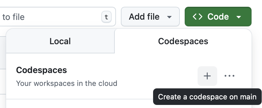
Fig. 3.11 Creating a new Codespace for your OER repository.#
To create a new Codespace, click on the green Butten “<> Code” in the top right corner of the repository page. Then click on the tab “Codespaces” and then the plus or “Create codespace on main”. This will create a new Codespace for your OER repository.
The creation of the Codespace will take a few minutes.
3.3.5. Exercise: Create a new Notebook#
You can either copy the empty Notebook assets/template_notebook.ipynb to the folder trust or you can create a new Notebook via the Codespace’s interface.
At the top of the page you can see a search bar (see Fig. 3.12).

Fig. 3.12 The search bar in the Codespace interface.#
In this search bar, you can search for files. You can also enter “command mode” by first typing a greather-than sign > and then searching for the command you want to use. As shown in Fig. 3.13, you can search for > jupyter to find the command to create a new Jupyter Notebook.
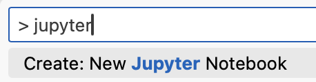
Fig. 3.13 The pallet in command mode
searching for > jupyter.#
This creates a new and unsaved Notebook (see Fig. 3.14).
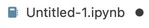
Fig. 3.14 New, unsaved Notebook as shown in tab bar.#
Exercise: Add a title and save the notebook file
Add a Markdown cell at the top of the Notebook and add a title to it.
Save the Notebook file with a meaningful name, e.g.
analyzing_data_on_trust.ipynb.
Solution
If you move your mouse between two cells, you can find buttons to add a new cell. Add a Markdown cell above the first cell. Add a title to the cell, e.g.
Analyzing Data on Trust.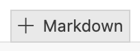
Either use the keyboard shortcut or the menu (see Fig. 3.15) to save the Notebook file. Choose a meaningful name, e.g.
analyzing_data_on_trust.ipynband don’t forget to specify the correct path. The file should be situated in the foldertrust.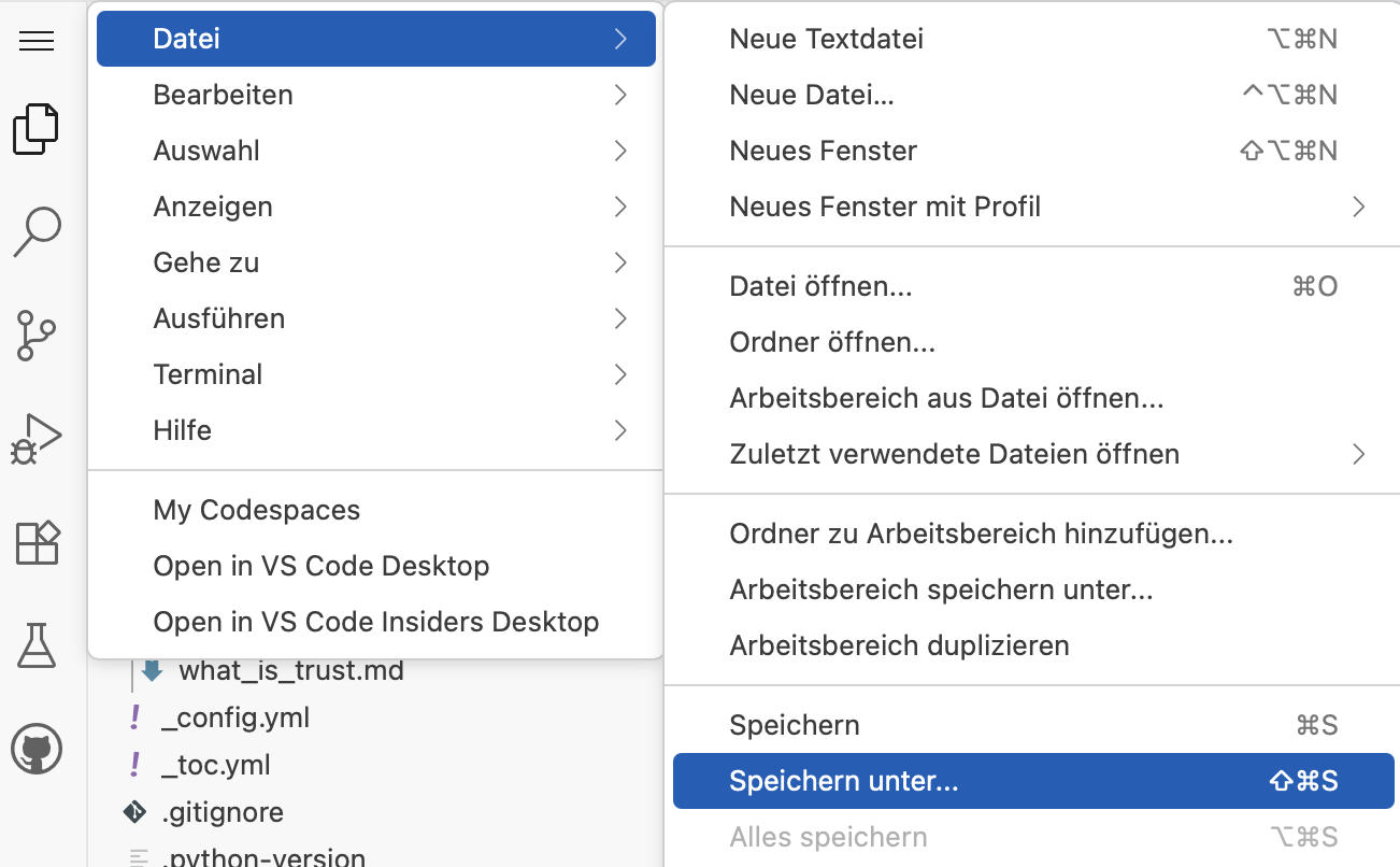
Fig. 3.15 The menu in the Codespace interface.#
3.3.6. Exercise: Using Python to analyze the data on trust#
In the following exercises, you will author a sample analysis of the dataset on Self-reported trust attitudes using Python code in the Notebook.
We will use a pre-processed version of the dataset, which you can download here in its latest version: cleaned_trust_data.csv.
Exercise: Loading the dataset
Add a code cell to the Notebook and import the necessary libraries. (Follow section 5.2.2)
Load the prepared dataset. (Follow Section 5.2.3)
Take a look at the dataset. Start with the following code snippet:
for i, observation in enumerate(survey_data[:5]):
    print(f"  {i+1}. {observation}")
Calculate one of the following values:
The number of Countries in the dataset.
The time span of the dataset.
The minimal and maximal trust values in the dataset. (Don’t forget the datatype conversion.)
Write a short explanation for learners using your OER.
Solution
See section 5.2.4 for a sample solution.
Exercise: Calculating statistical measures
Create a new section in your Notebook and add Python code to calculate the average trust level with the following code snippet:
trust_percentages = [float(obs['Trust_Percentage']) for obs in survey_data]
avg_trust = statistics.mean(trust_percentages)
print(f"Average trust level: {avg_trust:.1f}%")
Now add code to calculate at least one more of the following statistical measures:
Median trust level
Lowest trust level
Highest trust level
Total variation of trust levels
Standard deviation of trust levels
Add a section for learners of your OER. Which questions can you answer with those statistical measures?
Solution
See section 5.2.5 for a sample solution.
Also look at 5.2.6 for more advanced analyses.
Exercise: Creating a visualization
Go to section 5.2.7 and extract the code for one of the four visualizations. Add a code cell to your Notebook and paste the code there. Now play around with the code to change the visualization.
Also add a Markdown cell with a short explanation of the visualization and what it shows.
Solution
See section 5.2.7 for a sample solution.